Optimizing a code intelligence backend
When it comes to developer tools, speed is a critical feature. The difference between a 100ms, 1s, and 10s delay fundamentally alters user psychology—it's the difference between coding at the speed of thought vs. losing focus as your mind wanders while waiting for the UI to respond.
One of Sourcegraph's magic powers is its ability to provide compiler-accurate code navigation in completely web-based interfaces: Sourcegraph.com, private Sourcegraph instances, and on GitHub, GitLab, Bitbucket, and Phabricator via the Sourcegraph browser extension.
While compiler-level accuracy is great, one painpoint has been performance on larger codebases. The desire for speed motivated our switch from language servers to use of the Language Server Index Format (LSIF). Indexing vastly improves query latency by precomputing the data needed to serve doc tooltips, go-to-definition, and find-references requests, without sacrificing accuracy. Since adding support for LSIF, we've continued to optimize our code navigation backend. In Sourcegraph 3.16, we rewrote the LSIF processing backend from TypeScript to Go with the aim of optimizing performance. In 3.17, we made good on these plans.
With the guidance of the Go memory and CPU profiler, we implemented optimizations that fell into three areas:
- Architecture changes
- Parallelization
- Doing less stuff (where "stuff" is I/O, CPU usage, and memory allocations)
Identifying bottlenecks
Premature optimization is the root of all evil, so we initiated our optimization efforts by using a CPU and memory profiler to identify performance bottlenecks in our existing system. Here are the CPU and memory allocation profiles we began with:


These profiles revealed a number of hotspots in the code, and we combined these results with a high-level understanding of the system architecture to come up with a list of changes that would have a substantial impact on both upload and query performance.
These efforts yielded a 2x speedup in query latency, a 2x speedup in processing latency, and a nearly 50% reduction in memory and disk load. In this post, we'll highlight what impact each optimization had, and we'll dive into a detailed summary of overall improvements at the end.
Architecture changes
The CPU profiling revealed a substantial amount of time was being spent in the API server. This service receives the LSIF upload from the API user and passes it to the bundle manager server which writes it to disk. A separate background worker service later converts the on-disk LSIF data into a SQLite bundle. On a user query, the API server receives the requests, queries the bundle manager server, which in turn uses the SQLite bundle to respond to the API server, which then forwards that response to the user.
")
The "middleman" nature of the API server when serving user requests was an artifact of the initial architecture of the indexed precise code navigation system. After porting this system to Go in 3.16, it became apparent that the API server was a very thin wrapper around the bundle manager API, so in 3.17, we decided to remove it altogether.
")
The way we did this was a bit of a kludge. In essence, we wanted to eliminate an unnecessary network call between the precise code API server client (in the Sourcegraph frontend service) and the API server. However, we didn't want to have to write a bunch of new code to define an API service and client for the bundle manager directly, so what we did was we kept the existing API server and client as-is, but replaced the actual network calls with function calls to the HTTP handler functions directly.
In the code, we use the httptest.NewRecorder function to record the handler response, and then return this request to the caller as if it came from an actual over-the-network HTTP client call. Not the cleanest code in the world, but this addressed the immediate performance bottleneck and we were eager to move onto the others. In a separate pass, we were able to even further collapse this boundary and replace the fake HTTP server shim with direct function calls.
Parallelization
Overall, the entire process of converting an LSIF index into a bundle file is a simple, linear pipeline.
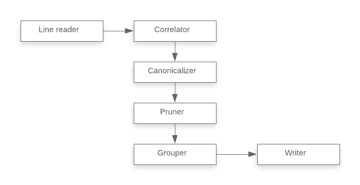
- The line reader reads raw LSIF input line-by-line and passes data to the correlator.
- The correlator builds an in-memory representation of the LSIF data and passes it to the canonicalizer.
- The canonicalizer deduplicates and denormalizes the in-memory representation.
- The pruner removes data that is not viewable within Sourcegraph (e.g., index data for uncommitted files).
- The grouper converts the in-memory representation to the format that will be stored on disk.
- The writer serializes this data to disk.
We identified that the reading and writing steps (marshalling, unmarshalling, and I/O) occupied the majority of time spent, which is where we focused our parallelization efforts.
Parallel JSON parsing
Profiling identified JSON parsing as a CPU hotspot, which pointed us to the reader portion of the pipeline. LSIF data is uploaded as JSON that describes the network of nodes and edges that captures the referential structure of code:
{"id":"13","type":"vertex","label":"definitionResult"}
{"id":"14","type":"edge","label":"textDocument/definition","outV":"11","inV":"13"}
{"id":"15","type":"edge","label":"item","outV":"13","inVs":["10"],"document":"7"}
{"id":"16","type":"vertex","label":"packageInformation","name":"github.com/sourcegraph/sourcegraph","manager":"gomod","version":"v3.17.0-rc.1-82e67052f048"}
During upload, the reader reads this data and parses it into JSON. We can split the raw JSON into different chunks that can be parsed in parallel (provided we remember to assemble the parsed results at the end in their original order). However, CPU time alone isn't a bulletproof indicator that optimizing a portion of a pipeline will decrease the latency of the pipeline overall. A CPU-intensive segment might very well be producing output faster than the next segment of the pipeline can consume (a fast producer, slow consumer scenario), in which case making the producer even faster would do us no good. To verify that this wasn't the case, we did a quick sanity check by disabling the next step of the pipeline (the correlator) and re-running the pipeline up to that point. This showed no improvement in overall time, which was consistent with the hypothesis that JSON parsing was indeed the bottleneck.
In the implementation, we used channels as bounded queues to break up the parsing into separate jobs that can be processed in parallel. The channel acts as a read-ahead buffer:
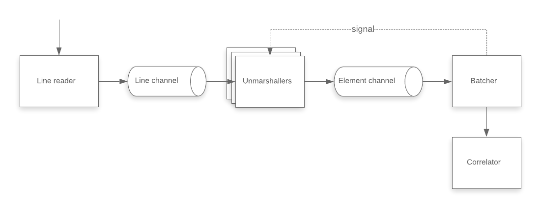
- The unmarshaller goroutines read lines from an input channel, parse it, and place the result into an output element channel.
- A batcher goroutine then consumes the items from the element channel in batches, reordering them by input ID to be consistent with the original order in the LSIF data.
- After the batch receives the expected number of values from the channel, it sends a signal to the unmarshallers to free them to resume work. This signalling procedure ensures that no unmarshaller looks for work past the current batching window (which would be pointless and wasteful).
- Each completed batch is then passed to the correlator for processing.
This update, implemented in 1e83fa6, reduced conversion time by 31%.
Writing to SQLite in parallel
The output of the LSIF processing system is a SQLite bundle that contains 4 categories of data:
- Document data includes a set of ranges for each code file that correspond to locations of definitions or references. The data also include the hover text for each range and pointers to other range identifiers (defined in result chunks).
- Result chunk data includes definition and reference range identifiers that are shared between documents. This data is sharded by a hashed identifier.
- Definition data is a lookup table for symbol occurrences by their export monikers.
- Reference data which acts as a lookup table for symbol occurrences by their import monikers.
To complete a go-to-definition or find-references action, we first load the document data for the current file path, find the range enclosing the user's cursor, and then look up the associated set of definition or reference identifiers. We then use these identifiers to look up the result ranges defined inside result chunks.
If we want to look up definitions or references by name, rather than cursor location, we can construct a partial moniker out of the name and look up definitions and references in the definition and reference data.
We optimized the time it took to write the SQLite bundle by taking advantage of the structure of these 4 categories of data. Prior to 3.17, the worker process would start four goroutines, one for each category, and would sequentially write batches of data into the target table. The SQLite batcher inserter utility is about as fast as it can be: it sets the correct pragmas, uses a single transaction, and minimizes the number of commands by squeezing as many rows into each insert statement as possible.
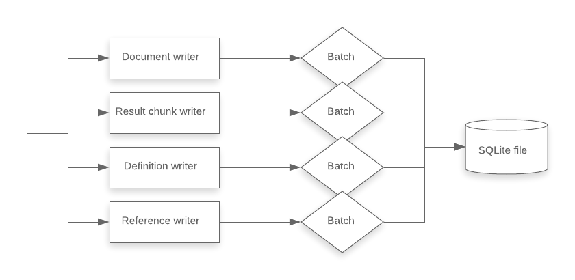
To increase write throughput, we moved the parallelism into the writer layer. After this change, document data, result chunk data, definition data, and reference data could be written to the bundle in sequence, but each write operation would send data to n batches in parallel. This more evenly distributes the serialize-and-write load across the available number of cores.
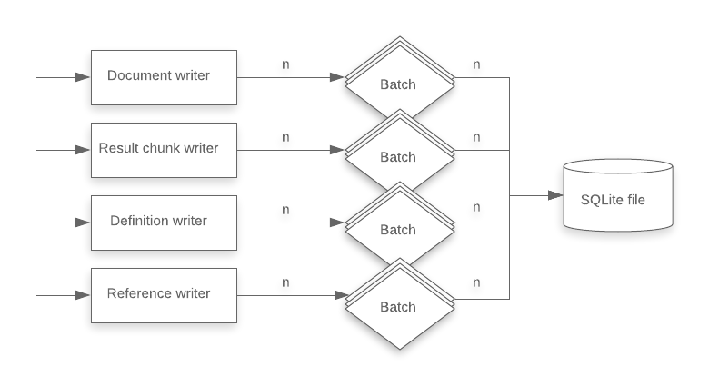
This update, implemented in 7c99cd9, reduced conversion time by 10.43%.
Other code changes: doing fewer things
In addition to simplifying the architecture and parallelizing critical tasks, we also made numerous targeted updates to be smarter (thriftier) to reduce the amount of data allocated in memory, serialized, and persisted.
Collapse rows in SQLite
Prior to Sourcegraph 3.17, each definition and reference mapped to its own row in the SQLite table. Each such row consisted of the following:
- An auto-generated numerical UUID
- LSIF moniker, composed of scheme and identifier (e.g.
gomodandgo.etcd.io/etcd/v3/raft:Ready) - A source location (file path, file offset range)
In total, this was 8 columns (1 for the UUID, 2 for the moniker, 5 for the location). An index on the schema and identifier columns enabled fast lookup by moniker. In a given codebase, there can be many millions of such rows.
Because there can be many references to a single definition, there will be many rows with duplicate values for the moniker, which means a lot of redundancy in the SQLite table. Since we are looking up by moniker anyway, it makes sense to group the data by moniker. In 3.17, we did just that, serializing all of the source locations associated with a particular moniker into a single compressed data blob. This greatly reduced the number of rows written to the database (and to column indexes).
The table below shows the number of definition and reference rows in each bundle file before and after this change in the set of repositories we used for integration testing. The decrease in the number of definition rows written grew proportionally with code size (yielding greater savings the larger the project), and the number of reference rows written decreased by an order of magnitude in all cases.
| repository | definition rows (before) | definition rows (after) | reference rows (before) | reference rows (after) |
|---|---|---|---|---|
| pingcap/tidb | 17,888 | 15,236 (-15%) | 32,2972 | 19,046 (-94%) |
| etcd-io/etcd | 9,862 | 9,279 (-6%) | 85,718 | 9,990 (-88%) |
| distributedio/titan | 1,082 | 1,016 (-6%) | 11,821 | 1,236 (-90%) |
| uber-go/zap | 967 | 902 (-7%) | 6,732 | 951 (-86%) |
Due to the reduced size of data, we are also able to insert more definition and references per SQL update query, further decreasing the overall time it takes to write a bundle. (SQLite imposes a hard insertion limit, SQLITE_MAX_VARIABLE_NUMBER.)
This update, implemented in 69bf52c, reduced bundle sizes by 50%.
Faster, smaller serialization
We replaced the gzipped JSON-encoded bundle payloads with gzipped gob-encoded structures. This reduced heap allocations, reduced overall bundle size, and yielded small improvements in overall processing time.
Most importantly, this allowed us to remove some tech debt caused by data structures that had evolved to become more complex over time. In particular, we used custom replacers to enable the serialization of TypeScript maps and sets, which we had to replicate in the Go rewrite in order to continue reading previously generated bundle files.
This update, implemented in d17750f, reduced bundle sizes by 10%.
Empty slice allocations
After porting the LSIF processing system from TypeScript to Go, our code was littered with empty slice allocations like this one:
rangePairs := []interface{}{}In Go, the size of a slice is tied to two fields: size and capacity. Size corresponds to the number of elements in the slice and capacity corresponds to the number of elements for which memory has been allocated in the slice. When the size exceeds the capacity, more memory must be allocated.
In Go, this is done by allocating a block of memory twice the size of the original and copying over the slice contents from the old memory block to the new one. This behavior does yield amortized constant time insertion, but the copying is expensive, and each memory block that is abandoned will need to be garbage collected at some point. This cost is exacerbated if the number of insertions into an originally empty slice is quite large, causing short-lived allocations to pile up.
If you can estimate the number of elements that will be inserted into the slice, you can save the runtime from a lot of intermediate allocations:
rangePairs := make([]interface{}, 0, len(d.Ranges))In our case, rewriting empty slice allocations to have non-zero capacities did not make a huge impact on overall performance, but it was easy to do and yielded better readability by making the purpose of new empty slices clearer.
This update, implemented in 8a905ac, reduced conversion time by 9.35%.
Maps vs. structs
In TypeScript, the most common associative data structure that maps from key to value is a JavaScript object ({}). The closest analog that Go has is a map from string to interface (map[string]interface{}). However, if the set of key values and the corresponding value types are known at compile time, Go has another data structure, the struct, which has different runtime characteristics.
After the rewrite from TypeScript to Go, the serialization code passed a map[string]interface{} instance to the json.Marshal function:
func (*defaultSerializer) MarshalDocumentData(d types.DocumentData) ([]byte, error) {
    // ...

    encoded, err := json.Marshal(map[string]interface{}{
        "ranges":             map[string]interface{}{"type": "map", "value": rangePairs},
        "hoverResults":       map[string]interface{}{"type": "map", "value": hoverResultPairs},
        "monikers":           map[string]interface{}{"type": "map", "value": monikerPairs},
        "packageInformation": map[string]interface{}{"type": "map", "value": packageInformationPairs},
    }

    // ...
}
In Sourcegraph 3.17, the map instances became typed struct instances:
type SerializingTaggedValue struct {
	Type  string      `json:"type"`
	Value interface{} `json:"value"`
}

func (*jsonSerializer) MarshalDocumentData(d types.DocumentData) ([]byte, error) {
    // ...

    encoded, err := json.Marshal(SerializingDocument{
        Ranges:             SerializingTaggedValue{Type: "map", Value: rangePairs},
        HoverResults:       SerializingTaggedValue{Type: "map", Value: hoverResultPairs},
        Monikers:           SerializingTaggedValue{Type: "map", Value: monikerPairs},
        PackageInformation: SerializingTaggedValue{Type: "map", Value: packageInformationPairs},
    }

    // ...
}
In Go, map values are allocated on the heap, while non-pointer struct instances are allocated on the stack. The switch from heap allocation to stack allocation for this data yielded substantial improvements in performance.
This update, implemented in 8a905ac, reduced conversion time by 9.35%.
Reducing data movement
The conventional wisdom holds that stack allocation is often more efficient than heap allocation, but this is not always the case. For example, there are cases where naive stack allocation will result in unnecessary copying. Consider the following for-loop, which is representative of a pattern that was quite common in our code:
resolvedLocations := make([]gql.LocationResolver, 0, len(locations))
for _, location := range locations {
    resolver, err := resolveLocation(ctx, locationResolver, location)
    if err != nil {
        return nil, err
    }
    if resolver == nil {
        continue
    }

    resolvedLocations = append(resolvedLocations, resolver)
}
The locations slice holds non-pointer struct values, each of which has around 20 fields. On each iteration of the loop, one of these values is copied into the portion of the stack allocated to hold the loop variable location. go-lint warns us about this:
rangeValCopy: each iteration copies 216 bytes (consider pointers or indexing) (gocritic) go-lintThis prompts a small, but significant change:
resolvedLocations := make([]gql.LocationResolver, 0, len(locations))
for i := range locations {
    resolver, err := resolveLocation(ctx, locationResolver, location[i])
    if err != nil {
        return nil, err
    }
    if resolver == nil {
        continue
    }

    resolvedLocations = append(resolvedLocations, resolver)
}
At runtime, this eliminates the need to copy the 216 bytes of each slice element into an intermediate location variable before copying it again into the activation record of the resolveLocation function call.
This update, implemented in d1f8caf, reduced conversion time by 26.18%.
Efficient JSON parsing
The Go standard library's JSON parser is reliable and has an easy-to-use API. However, it is not hyper-optimized for performance. Profiling showed that the most CPU time in the correlation phase of processing was spent in the "encoding/json" package, due to its heavy use of reflection.
We looked at several other options for JSON parsing in Go (easyjson, fastjson, ffjson) before finally settling on json-iterator/go, a high-performance drop-in replacement for the standard library's encoding/json package. The low switching cost and the efficiency of decoding small structures (which are common in LSIF vertex and edge definitions) were the key considerations that motivated our choice.
This update, implemented in 6b12b26, reduced conversion time by 19.02%.
Avoid unnecessary disk writes
The bundle manager acts as a sort of hub in the code navigation backend system, fetching LSIF data and serving it to workers, which then convert it into SQLite bundles that are then passed back to the bundle to write to disk.
Previously, when a worker requested LSIF data, the bundle manager would request the data using an HTTP request, write it to disk, and then pass the filename to the worker process.
This disk-write turned out to be unnecessary, as we could simply pass the HTTP response reader back to the worker directly. Not only did this eliminate the need to write the data out to disk, it also enabled a streaming data processing model, as the worker could begin consuming the data from the HTTP response reader without blocking on serializing the entire data structure.
This yielded a performance boost that became more significant the larger the codebase and corresponding LSIF data.
This update, implemented in 2eae464, reduced conversion time by 20.13%.
Reviewing results
The following chart shows the decrease in query latency while running our integration test suite compared to the previous two Sourcegraph releases. The test suite is querying cross-repo definitions and references over three commits from etcd-io/etcd, pingcap/tidb, and distributedio/titan, and two commits from uber-go/zap.

This next chart shows the time required to upload and process the indexes.

These last charts show the size of the converted bundle on disk after conversion.
 size on disk chart")
 size on disk chart")
 size on disk chart")
 size on disk chart")
With all the changes discussed in this post combined, the latency for queries and upload processing has been cut by a factor of two, as has the size of bundles on disk, compared to Sourcegraph 3.15.
Finally, here are the before and after profiles of CPU, memory allocations, and heap of the LSIF processing system. Note that most of the original red spots have been eliminated. New ones have naturally emerged, but overall the system is much faster:


We plan to continue on this path of performance improvements, and the next release will focus specifically on processing multiple bundles in parallel in order to multiply the benefit of these recent performance gains. This is just the latest chapter in our continuing effort to bring fast, precise code navigation to every language, every codebase, and every programmer. If you thought this post was interesting or valuable, we'd appreciate it if you'd share it with others!